GRACE TECHNICAL REPORTS
Marker-directed Optimization of UnCAL
Graph Transformations (revised version)
Soichiro Hidaka
Zhenjiang Hu
Kazuhiro Inaba
Hiroyuki Kato
Kazutaka Matsuda
Keisuke Nakano
Isao Sasano
GRACE-TR 2011–06
November 2011
CENTER FOR GLOBAL RESEARCH IN
ADVANCED SOFTWARE SCIENCE AND ENGINEERING
NATIONAL INSTITUTE OF INFORMATICS
2-1-2 HITOTSUBASHI, CHIYODA-KU, TOKYO, JAPAN
Marker-directed Optimization of UnCAL Graph
Transformations
!Soichiro Hidaka1, Zhenjiang Hu1, Kazuhiro Inaba1, Hiroyuki Kato1, Kazutaka Matsuda2, Keisuke Nakano3, and Isao Sasano4
1
National Institute of Informatics, Japan,
{hidaka, hu, kinaba, kato}@nii.ac.jp
2
The University of Electro-Communications, Japan,
3 Tohoku University, Japan,
4
Shibaura Institute of Technology, Japan,
Abstract. Buneman et al. proposed a graph algebra called UnCAL (Un-structured CALculus) for compositional graph transformations based on structural recursion, and we have recently applied to model transfor-mations. The compositional nature of the algebra greatly enhances the modularity of transformations. However, intermediate results generated between composed transformations cause overhead. Buneman et al. pro-posed fusion rules that eliminate the intermediate results, but auxiliary rewriting rules that enable the actual application of the fusion rules are not apparent so far. UnCAL graph model includes the concept of mark-ers, which correspond to recursive function call in the structural recur-sion. We have found that there are many optimization opportunities at rewriting level based on static analysis, especially focusing on markers. The analysis can safely eliminate redundant function calls. Performance evaluation shows its practical effectiveness for non-trivial examples in model transformations.
Keywords:program transformations, graph transformations, UnCAL
1
Introduction
Graph transformation has been an active research topic [8] and plays an impor-tant role in model-driven engineering [5, 10]; models such as UML diagrams are
!This is a revised version of the technical report: Soichiro Hidaka, Zhenjiang
represented as graphs, and model transformation is essentially graph transfor-mation. We have recently proposed a bidirectional graph transformation frame-work [6] based on providing bidirectional semantics to an existing graph transfor-mation language UnCAL [4], and applied it to bidirectional model transforma-tion by translating from existing model transformatransforma-tion language to UnCAL [9]. Our success in providing well-behaved bidirectional transformation framework was due to structural recursion in UnCAL, which is a powerful mechanism of visiting and transforming graphs. Transformation based on structural recursion is inherently compositional, thus facilitates modular model transformation pro-gramming.
However, compositional programming may lead to many unnecessary inter-mediate results, which would make a graph transformation program terribly in-efficient. As actively studied in programming language community, optimization like fusion transformation [11] is desired to make it practically useful. Despite a lot of work being devoted to fusion transformation of programs manipulating lists and trees, little work has been done on fusion on programs manipulating graphs. Although the original UnCAL has provided some fusion rules and rewrit-ing rules to optimize graph transformations [4], we believe that further work and enhancement on fusion and rewriting are required.
The key idea presented in this paper is to analyze input/output markers, which are sort of labels on specific set of nodes in the UnCAL graph model and are used to compose graphs by connecting nodes with matching input and output markers. By statically analyzing connectivity of UnCAL by our marker analysis, we can simplify existing fusion rule. Consider, for instance, the following existing generic fusion rule of the structural recursion operator in UnCAL:
rec(λ($l2,$t2).e2)(rec(λ($l1,$t1).e1)(e0))
=rec(λ($l1,$t1).rec(λ($l2,$t2).e2)(e1@rec(λ($l1,$t1).e1)($t1)))(e0) where rec(λ($l,$t).e) applies transformation e on each edge (whose label is bound to $l and subgraph pointed by the edge is bound to $g) of the input graph, and combine the results ofeto produce the output graph.recencodes a structural recursive function which is an important computation pattern and ex-plained later. The graph constructor@connects two graphs by matching markers on nodes, and in this case, result of transformation e1 is combined to another structural recursion rec(λ($l1,$t1).e1). If we know by static analysis that e1 creates no output markers, or equivalently, rec(λ($l1,$t1).e1) makes no recur-sive function call, then we can eliminate @rec(λ($l1,$t1).e1)($t1) and further simplify the fusion rule. Our preliminary performance analysis reports relatively good evidence of usefulness of this optimization.
The main technical contributions of this paper are two folds:
1
2 a
3 b
4 c
5 a a
c
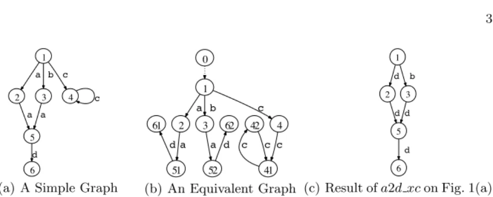
6 d
(a) A Simple Graph
0
1
2
a
3
b
4
c
51
a
61
52
a
62
41
c
42
c
d d c
(b) An Equivalent Graph (c) Result ofa2d xcon Fig. 1(a)
Fig. 1.Graph Equivalence Based on Bisimulation
over-approximation missed the chance of expression simplification exempli-fied above. Our inference can avoid this over-approximation by avoiding subtyping rule and computing the sets in a bottom-up manner.
– A set of rewriting rules for optimization using inferred markers (Section 4), that is more powerful than that in [4] in the sense that more expressions are simplified as exemplified above.
All have been implemented and tested with graph transformations widely recog-nized in software engineering research. The source code of the implementation can be downloaded via our project web site atwww.biglab.org.
The rest of this paper is organized as follows. Section 2 reviews UnCAL graph model, graph transformation language and existing optimizations. Sec-tion 3 proposes enhanced static analysis of markers. In SecSec-tion 4, we build en-hanced rewriting optimization algorithm based on the static analysis. Section 5 reports preliminary performance results. Section 6 reviews related work, and Section 7 concludes this paper.
2
UnCAL Graph Algebra and Prior Optimizations
In this section, we review the UnCAL graph algebra [3, 4], in which our graph transformation is specified.
2.1 Graph Data Model
We deal with rooted, directed, and edge-labeled graphs with no order on outgoing edges. They are edge-labeled in the sense that all information is stored on labels of edges while nodes have no labels. UnCAL graph data model has two prominent features, markers and ε-edges. Nodes may be marked with input and output markers, which are used as an interface to connect them to other graphs. An
Formally, a graph G, sometimes denoted by G(V,E,I,O), is a quadruple (V, E, I, O), where V is a set of nodes, E ⊆ V ×(Label ∪ {ε})×V is a set of edges,I⊆ M ×V is a set of pairs of an input marker and the corresponding node, andO⊆V × Mis a set of pairs of nodes and associated output markers. For each marker&x ∈ M, there is at most one nodev such that (&x, v)∈I. The node v is called aninput nodewith marker &x and is denoted by I(&x). Unlike input markers, more than one node can be marked with an identical output marker. They are calledoutput nodes. Intuitively, input nodes are root nodes of the graph (we allow a graph to have multiple root nodes, and for singly rooted graphs, we often use default marker&to indicate the root), while an output node can be seen as a “context-hole” of graphs where an input node with the same marker will be plugged later. We writeinMarker(G) to denote the set of input markers andoutMarker(G) to denote the set of output markers in a graphG.
Note that multiple-marker graphs are meant to be an internal data struc-ture for graph composition. In fact, the initial source graphs of our trans-formation have one input marker (single-rooted) and no output markers (no holes). For instance, the graph in Fig. 1(a) is denoted by (V, E, I, O) where
V = {1,2,3,4,5,6}, E = {(1,a,2),(1,b,3),(1,c,4),(2,a,5),(3,a,5),(4,c,4),
(5,d,6)}, I = {(&,1)}, and O = {}. DBXY denotes graphs with sets of input markersX and output markersY. DB{Y&}is abbreviated to DBY.
2.2 Notion of Graph Equivalence
Two graphs are value equivalent if they are bisimilar. Please refer to [4] for the complete definition. Informally, graphG1 is bisimilar to graphG2 if every node
x1 in G1 has at least a bisimilar counterpart x2 in G2 and vice versa, and if there is an edge fromx1 to y1 in G1, then there is a corresponding edge from
x2 to y2 in G2 that is a bisimilar counterpart ofy1, and vice versa. Therefore, unfolding a cycle or duplicating shared nodes does not really change a graph. This notion of bisimulation is extended to cope with ε-edges. For instance, the graph in Fig. 1(b) is value equivalent to the graph in Fig. 1(a); the new graph has an additional ε-edge (denoted by the dotted line), duplicates the graph rooted at node 5, and unfolds and splits the cycle at node 4. Unreachable parts are also disregarded, i.e., two bisimilar graphs are still bisimilar if one adds subgraphs unreachable from input nodes.
This value equivalence provides optimization opportunities because we can rewrite transformation so that transformation before and after rewriting produce results that are bisimilar to each other [4]. For example, optimizer can freely cut off expressions that is statically determined to produce unreachable parts.
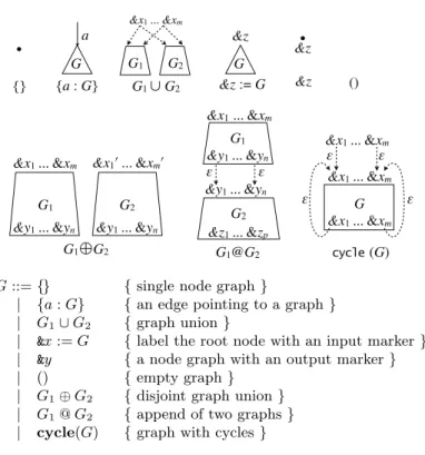
2.3 Graph Constructors
G::={} {single node graph}
| {a:G} {an edge pointing to a graph} | G1∪G2 {graph union}
| &x:=G {label the root node with an input marker} | &y {a node graph with an output marker} | () {empty graph}
| G1⊕G2 {disjoint graph union}
| G1@G2 {append of two graphs}
| cycle(G) {graph with cycles}
Fig. 2.Graph Constructors
label a ∈ Label∪ {ε} pointing to the root of graph G, and G1∪G2 adds two
ε-edges from the new root to the roots of G1 andG2. Also,&x :=Gassociates an input marker,&x, to the root node ofG,&y constructs a graph with a single node marked with one output marker&y, and () constructs an empty graph that has neither a node nor an edge. Further,G1⊕G2 constructs a graph by using a componentwise (V, E, I and O) union. ∪differs from ⊕ in that∪ unifies input nodes while ⊕does not. ⊕ requires input markers of operands to be disjoint, while ∪requires them to be identical.G1@G2 composes two graphs vertically by connecting the output nodes of G1 with the corresponding input nodes of
G2withε-edges, andcycle(G) connects the output nodes with the input nodes of G to form cycles. Formal definitions can be found in the full version of [6]. The definition here is based on graph isomorphism (identical graph construc-tion expressions results in identical graphs up to isomorphism), and they are, together with other operators, also bisimulation generic [4], i.e., bisimilar result is obtained for bisimilar operands.
Example 1. The graph equivalent to that in Fig. 1(a) can be constructed as follows (though not uniquely).
&z@cycle((&z :={a:{a:&z1}} ∪ {b:{a:&z1}} ∪ {c:&z2})
⊕(&z1:={d:{}})
e::= {} | {l:e} |e∪e|&x :=e|&y|()
| e⊕e|e@e|cycle(e) {constructor}
| $g {graph variable}
| let$g=eine { variable binding} | ifl=ltheneelsee {conditional} | rec(λ($l,$g).e)(e) {structural recursion application}
l ::= a|$l {label (a∈Label) and label variable}
Fig. 3.Core UnCAL Language
For simplicity, we often write{a1 : G1, . . . , an :Gn} to denote {a1 :G1} ∪
· · · ∪ {an:Gn}, and (G1, . . . , Gn) to denote (G1⊕ · · · ⊕Gn).
2.4 UnCAL Syntax
UnCAL (Unstructured CALculus) is an internal graph algebra for the graph query language UnQL, and its core syntax is depicted in Fig. 3. It consists of the graph constructors, variables, variable bindings (letis our extension and is used for rewriting), conditionals, and structural recursion. We have already detailed the data constructors, while variables, variable bindings and conditionals are self explanatory. Therefore, we will focus onstructural recursion, which is a powerful mechanism in UnCAL to describe graph transformations.
A functionf on graphs is called astructural recursionif it is defined by the following equations
f({}) ={}
f({$l: $g}) =e@f($g)
f($g1∪$g2) =f($g1)∪f($g2),
andf can be encoded byrec(λ($l,$g).e). Despite its simplicity, the core UnCAL is powerful enough to describe interesting graph transformation including all graph queries (in UnQL) [4], and nontrivial model transformations [7].
Example 2. The following structural recursion a2d xcreplaces all labelsawith dand removes edges labeledc.
a2d xc($db) =rec(λ($l,$g).if$l=athen {d:&}
else if$l=cthen{ε:&}
else {$l:&}) ($db)
The outerif of the nestedifs corresponds toein the above equations. Applying the functiona2d xcto the graph in Fig. 1(a) yields the graph in Fig. 1(c). &'
2.5 Revisiting Original Marker Analysis
technical report version of [2]. Note that we call type to denote sets of input and output markers. Compared to our analysis, these rules were provided declara-tively. For example, the rule for if says that if sets of output markers in both branches are equal, then the result have that set of output markers. It is not apparent how we obtain the output marker of if if the branches have different sets of output markers.
Buneman et al. [4] did mention optimization based on marker analysis, to avoid evaluating unnecessary subexpressions. But it was mainly based on run-timeanalysis. As we propose in the following sections, we canstaticallycompute the set of markers and further simplify the transformation itself.
2.6 Fusion Rules and Output Marker Analysis
Buneman et al. [3, 4] proposed the following fusion rules that aim to remove intermediate results in successive applications of structural recursionrec.
rec(λ($l2,$t2).e2)(rec(λ($l1,$t1).e1)(e0))
=
rec(λ($l1,$t1).rec(λ($l2,$t2).e2)(e1))(e0) if $t2 does not appear free ine2
rec(λ($l1,$t1).rec(λ($l2,$t2).e2)
(e1@rec(λ($l1,$t1).e1)($t1)))(e0) for arbitrarye2
(1) If you can statically guarantee that e1 does not produce any output marker, which means therecis “non-recursive”, then the second rule is promoted to the first rule, opening another optimization opportunities.
Non-recursive Query. Now questions that might be asked would be how often do such kind of “non-recursive” queries appear. Actually it frequently appears as
extractionorjoin. Extraction transformation is a transformation in which some subgraphs are simply extracted. It is achieved by direct reference of the bound graph variable in the body ofrec. Join is achieved by nesting of these extraction transformations. Finite steps of edge traversals are expressed by this nesting.
Example 3. The following structural recursion consecutive extracts subgraphs that can be accessible by traversing two connected edges of the same label.
consecutive($db) =rec(λ($l,$g).rec(λ($l!,$g!).
if$l= $l!then{result: $g!}
else {} )($g))($db)
For example, we haveconsecutive
$
•a!!•X!!• ◦
a "
"
! !
b ## " "
•a!!•Y!!• %
=◦ result !!• X!!•.
&x:= (&z:=e)−→&x.&z:=e &x:= (e1⊕e2)−→(&x:=e1)⊕(&x:=e2)
e∪ {} −→e {} ∪e−→e e⊕()−→e ()⊕e−→e
() @e−→() e::DB X
Y X ∩ Y=φ
cycle(e)−→e
Fig. 4.Auxiliary Rewriting Rules
2.7 Other Prior Rewriting Rules
Apart from fusion rules, the following rewriting rules forrecare proposed in [4] for optimizations. Type ofeis assumed to beDBZZ. They simplify the argument ofrecand increase chances of fusions.
rec(λ($l,$t).e)({}) =1&
&z∈Z&z :={}
rec(λ($l,$t).e)({l:d}) =e[l/$l][d/$t]@rec(λ($l,$t).e)(d)
rec(λ($l,$t).e)(d1∪d2) =rec(λ($l,$t).e)(d1)∪rec(λ($l,$t).e)(d2)
rec(λ($l,$t).e)(&x :=d) =&x :=2(rec(λ($l,$t).e)(d))
rec(λ($l,$t).e)(&x) =&
&z∈Z&z :=&y.&z
rec(λ($l,$t).e)() = ()
rec(λ($l,$t).e)(d1⊕d2) =rec(λ($l,$t).e)(d1)⊕rec(λ($l,$t).e)(d2) The first rule eliminatesrec, while the second rule eliminates an edge from the argument.
$t does not occur free ine
rec(λ($l,$t).e)(d1@d2) =rec(λ($l,$t).e)(d1)@rec(λ($l,$t).e)(d2) $t does not occur free ine
rec(λ($l,$t).e)(cycle(d)) =cycle(rec(λ($l,$t).e)(d))
Additional rules proposed by (full version of) Hidaka et al. [7] to further simplify the body ofrecare given in Fig. 4. The rules in the last line in Fig. 4 can be generalized by static analysis of the marker in the following section. And given the static analysis, we can optimize further as described in Section 4.
3
Enhanced Static Analysis
This section proposes our enhanced marker analysis. Figure 5 shows the proposed marker inference rules for UnCAL. Dot notation (·) between markers and sets of markers represents “concatenation” of markers that satisfies the properties at the top of the figure. Static environment Γ denotes mapping from variables to their types. We assume that the types of free variables are given. Since we focus on graph values, we omit rules for labels. Roughly speaking,DBXY is a type for graphs that haveX input markers exactly and have at mostY output markers, which will be shown formally by Lemma 1.
1
Original right hand side was{}in [4], but we corrected here. 2
(&x·&y)·&z=&x·(&y·&z) &·&x=&x·&=&x X · Ydef= {&x·&y|&x∈ X,&y∈ Y}
Γ ' {}::DB∅
Γ 'l::Label
Γ 'e::DBY
Γ ' {l:e}::DBY
Γ 'e1::DBXY1
Γ 'e2::DBXY2
Γ 'e1∪e2::DBXY1∪Y2
Γ '() ::DB∅∅
Γ 'e::DBZ Y
Γ '&x :=e::DB{&x}·ZY Γ '&y::DB{&y}
Γ 'e1::DBX1Y1 Γ 'e2::DBX2Y2
X1∩ X2 =∅
Γ 'e1⊕e2 ::DBX1∪X2Y1∪Y2
Γ 'e1::DBX1Y1
Γ 'e2::DBX2Y2
Γ 'e1@e2::DBX1Y2
5 Γ 'e::DB X Y
Γ 'cycle(e) ::DBXY\X
Γ($g) =DBXY
Γ '$g::DBXY
Γ 'ea::DBXY
Γ{$l)→Label,$g)→DBY} 'eb::DBZZio Z=Zi∪ Zo
Γ 'rec(λ($l,$g).eb)(ea) ::DBX ·ZY·Z
Γ 'l1::Label Γ 'l2::Label
Γ 'et::DBXYt Γ 'ef::DBXYf
Γ 'ifl1=l2thenetelseef::DBXYt∪Yf
Γ 'e1::DBX1Y1
Γ{$g)→DBX1Y1} 'e2::DBX2Y2
Γ 'let$g=e1ine2::DBX2Y2
Fig. 5.UnCAL Static Typing (Marker Inference) Rules: Rules forLabelare Omitted
The original typing rules were provided based on the subtyping rule
Γ )e::DBXY Y ⊆ Y!
Γ )e::DBXY!
and required the arguments of∪,⊕,if to have identical sets of output markers. Unlike the original rules, the proposed type system does not use the subtyping rule directly for inference. Combined with the forward evaluation semanticsF[[]] that is summarized in [6], we have the following type safety property.
Lemma 1 (Type Safety). Assume that g is the graph obtained byg =F[[e]]
for an expression e. Then, ) e :: DBXY implies both inMarker(g) = X and
outMarker(g)⊆ Y.
Lemma 1 guarantees that the set of input markers estimated by the type infer-ence is exact in the sense that the set of input markers generated by evaluation exactly coincides with that of the inferred type. For the output markers, the type system provides an over-approximation in the sense that the set of output
5
markers generated by evaluation is a subset of the inferred set of output markers. Since the treatment of the input markers are identical to that in [4], we focus that on the output markers and prove it. The proof, which is based on induction on the structure of UnCAL expressions, is in Sect. A.2 in the appendix.
Between the original typing rules in [4], the following property holds: for all
X and Y, e :: DBXY for some Y! ⊇ Y if and only if e has a type DBX Y! in the original type system. The proof can be conducted by simple induction on the structure of the UnCAL expressions and appears in Sect. A.3 of the appendix.
4
Enhanced Rewiring Optimization
This section proposes enhanced rewriting optimization rules based on the static analysis shown in the previous section.
4.1 Rule for @ and Revised Fusion Rule
Statically-inferred markers enable us to optimize expressions much more. We can generalize, for example, the rewriting rule ()@e −→() in the last row of Fig. 4 to the following, by not just referring to the pattern of subexpressions but its estimated markers.
e1::DBX∅
e1@e2−→e1 (2)
As we have seen in Sect. 2, we have two fusion rules (1) forrec. Although the first rule can be used to gain performance, the second rule is more complex so less performance gain is expected. Using (2), we can relax the first condition of the fusion rule (1) to increase chances to apply the first rule as follows.
rec(λ($l2,$t2).e2)(rec(λ($l1,$t1).e1)(e0)) =rec(λ($l1,$t1).rec(λ($l2,$t2).e2)(e1))(e0)
if $t2 does not appear free ine2, or e1::DBX∅
Here, the underlined part is added to relax the entire condition.
4.2 Further Optimization with Static Marker Information
In this section, general rules fore1@e2 is investigated. First to eliminate@e2, and then to statically compute @by plugging e2into e1.
4.2.1 Static Output Marker Removal Algorithm and Soundness
For more general cases of@where connections byεdo not happen, we have the following rule.
e1::DBXY1 e2::DB
Y2
RmY//e00denotes static removal of the set of output markers, i.e., if)e::DBXY,
then ) RmW//e00 :: DBXY\W. Without this, rewriting result in spurious output
markers from e1 remained in the final result. The formal definition of RmY//e00 is shown below.
Rm∅//e00=e RmX ∪Y//e00=RmY//RmX//e0000 RmY//{}00={}
RmY//()00= () Rm{&y}//&y00={} Rm{&y}//&x00=&x
RmY//e11e200=RmY//e100 1RmY//e200 (1 ∈ {∪,⊕}) RmY//&x:=e00= (&x:=RmY//e00)
RmY//{l:e}00={l:RmY//e00}
RmY//e1@e200=e1@RmY//e200
RmY//ifbthene1elsee200=ifbthenRmY//e100elseRmY//e200
Since the output markers of the result ofe1@e2 are not affected by those ofe1,
e1is not visited in the rule of@. In the following,IdY andBotY are respectively defined as&
&z∈Y&z :=&z and
&
&z∈Y&z :={}.
e::DBXY &y ∈(Y \ X) Rm{&y}//e00=e!
Rm{&y}//cycle(e)00=cycle(e!)
e::DBXY &y ∈/(Y \ X) Rm{&y}//cycle(e)00=cycle(e)
$v ::DBXY &y ∈ Y/
Rm{&y}//$v00= $v
$v::DBXY &y ∈ Y
Rm{&y}//$v00= $v@(Bot{&y} ⊕IdY\{&y})
The first rule of $v says that according to the safety of type inference, &y is guaranteed not to result at run-time, so the expression $v remains unchanged. The second rule actually removes the output marker&yj, but static removal is impossible. So the removal is deferred till run-time. The output node marked&yj is connected to node produced by&y :={}. Since the latter node has no output marker, the original output marker disappears from the graph produced by the evaluation. The rest of the &yk :=&yk does no operation on the marker. Since estimationYis the upper bound, the output maker may not be produced at run-time. If it is the case, connection withε-edge by@does not occur, and the nodes produced by the := expressions are left unreachable, so the transformation is still valid. As another side effect, @ may connect identically marked output nodes to single node. However, the graph before and after this “funneling” connection are bisimilar, since every leaf node with identical output markers are bisimilar by definition. Should the output nodes are to be further connected to other input nodes, the target node is always single, because more than one node with identical input marker is disallowed by the data model. So this connection does no harm. Note that the second rule increases the size of the expression, so it may increase the cost of evaluation.
Forrec, one output marker&y ineacorresponds to{&y} · Z={&y.&z |&z ∈ Z} in the result. So removal of &y from ea results in removal of all of the{&y} · Z. So only removal of all of{&y.&z |&z ∈ Z}at a time is allowed.
Lemma 2 (Soundness of Static Output-Marker Removal Algorithm).
Assume that G = (V, E, I, O) is a graph obtained by G= F[[e]] for an expres-sion e, and e! is the expression obtained by RmY//e00. Then, we have F[[e!]] = (V, E, I,{(v,&y)∈O|&y ∈ Y}/ ).
Lemma 2 guarantees that no output marker inYappears at run-time ifRmY//e00 is evaluated.
4.2.2 Plugging Expression to Output Marker Expression
The following rewriting rule is to plug an expression into another through cor-respondingly marked node.
{l:&y}@ (&y:=e)−→ {l:e}
This kind of rewriting was actually implicitly used in the exemplification of optimization in [4], but was not generalized. We can generalize this rewriting as
e@ (&y:=e!)−→ '
RmY\{&y}//e00[e!/&y] if&y∈ Y wheree::DBXY
RmY//e00 otherwise.
where e[e!/&y] denotes substitution of &y bye! ine. Since nullrary constructors
{}, (), and &x 2= &y do not produce output marker &y, the substitution takes no effect and the rule in the latter case apply. So we focus on the former case in the sequel. For most of the constructors the substitution rules are rather straightforward:
&y[e/&y] =e
(e11e2)[e/&y] = (e1[e/&y])1(e2[e/&y]) (1 ∈ {∪,⊕}) (&x:=e)[e!/&y] = (&x:= (e[e!/&y]))
{l:e}[e!/&y] ={l: (e[e!/&y])}
(e1@e2)[e/&y] =e1@ (e2[e/&y])
(ifbthene1elsee2)[e/&y] =ifbthen(e1[e/&y])else(e2[e/&y])
Since the final output marker for@is not affected by that ofe1,e1is not visited in the rule of@. Forcycle, we should be careful to avoid capturing of marker.
cycle(e)[e!/&y] =
'
cycle(e[e!/&y]) if (Y!∩ X) =∅wheree::DBX
Y e!::DBY!
cycle(e)[e!/&y] otherwise.
in X, then the renaming is necessary. As suggested in the full version of [3], markers inX instead of those inY! should be renamed. And that renaming can be compensated outside ofcycleas follows:
cycle(e)def= ((
&x∈X
&x:=&tmpx) @cycle(e[&tmpx1/&x
1]. . .[&tmpxM/&xM])
where &x1, . . . ,&xM = X are the markers to be renamed, and X of e :: DBXY is used. Note that in the renaming, not only output markers, but also input markers are renamed. &tmpx1, . . . ,&tmpxM are corresponding fresh (temporary)
markers. The left hand side of@recovers the original name of the markers. After renaming bycycle, no marker is captured anymore, so substitution is guaranteed to succeed. For variable reference and rec, static substitution is impossible. So we resort to the following generic “fall back” rule.
e∈ {$v,rec( )( )} e::DBXY Y={&y1, . . . ,&yj, . . . ,&yn}
e[e!/&yj] =e@
)
&y1:=&y1, . . . ,&yj−1:=&yj−1,&yj:=e!, &yj−1:=&yj−1, . . . ,&yn:=&yn
*
The “fall back” rule is used for rec because unlike output marker removal algorithm, we can not just plug e into ea since that will not plug e but
rec(λ($l,$t).eb)(e) in the result. We could have used the inverserec(λ($l,$t).eb)−1 to plugrec(λ($l,$t).eb)−1(e!) instead, but the inverse does not always exist in general.
The overall rewriting is conducted by two mutually recursive functions as follows: a driver function first applies itself to subexpressions recursively, and then applies a function that implements−→and other rewriting rules recursively such as fusions described in this paper, on the result of the driver function. The implemented rewriting system is deterministic by imposing consistent order of rule applications by these functions.
With respect to proposed rewriting rules in this section, the following theorem holds.
Theorem 1 (Soundness of Rewriting). If e −→e!, thenF[[e]] is bisimilar
toF[[e!]].
It can be proved by simple induction on the structure of UnCAL expressions, and omitted here.
Example 4. The following transformation that apply selection afterconsecutive
in Example 3
rec(λ($l1,$g1).if$l1=athen{$l1: $g1}else{})(consecutive($db)) is rewritten as follows:
= {expand definition ofconsecutive and apply 2nd fusion rule}
rec(λ($l,$g).rec(λ($l1,$g1).if$l1=athen{$l1: $g1}else{}) (rec(λ($l!,$g!).if$l = $l! then{result: $g!}else{})($g)
@rec(λ($l,$g).rec(λ($l!,$g!).
= {(2)}
rec(λ($l,$g).rec(λ($l1,$g1).if$l1=athen{$l1: $g1}else{}) (rec(λ($l!,$g!).if$l = $l! then{result: $g!}else{})($g)))($db) = {2nd fusion rule, (2),recrule forif and{l:d}, static label comparison}
rec(λ($l,$g).rec(λ($l!,$g!).{})($g))($db)
This example demonstrates the second fusion rule promotes to the first. The top level edges of the result ofconsecutive are always labeled resultwhile the selection selects subgraphs under edges labeled a. So the result will always be empty, and correspondingly the body ofrecin the final result is{}. &'
More examples can be found in Sect. A.4 in the appendix.
The following remark summarizes how far can we remove intermediate graphs. Proof can be found in Section A.5 in the appendix.
Remark 1 (Removal of Intermediage Graph).Suppose we have a composition of the form
rec(λ($l2,$t2).e2)(C[rec(λ($l1,$t1).e1)(e0)])
whereC[] denotes context using constructors and if expressions. Then, (i) if $t2 does not appear free in e2, then the composition of the above form, including the ones that are generated during fusion, are removed. (ii) if $t2 appears free in e2 but e1 ::DB∅, and e1 consists of nestedrecwith context not using@ or
cyclewith body of typeDB∅, then the composition, including the ones that are generated during the fusion rule application, are removed.
5
Implementation and Performance Evaluation
This section reports preliminary performance evaluations. All of the transfor-mations in the paper are implemented in GRoundTram, or Graph Roundtrip Transformation for Models, which is a system to build a bidirectional transfor-mation between two models (graphs). All the source codes are available online at www.biglab.org. The following experimental results are obtained by the system. Performance evaluation was conducted onGRoundTram, running on MacOSX over MacBookPro 17 inch, with 3.06 GHz Intel Core 2 Duo CPU. An UnCAL transformation runs in time exponential to the size (number of compositions or nesting of recs) of the transformation (and polynomial to the size of input graph [4]). Thus, the proposed rewriting, which can reduce the size of transfor-mation, may change the elapsed time drastically even for the small graphs (up to a hundred of nodes) used in the experiments.
Table 1 shows the experimental results. Each running time includes time for forward and backward6 transformations [6], and for backward transforma-tions, algorithm for edge-renaming is used, and no modification on the target is
6
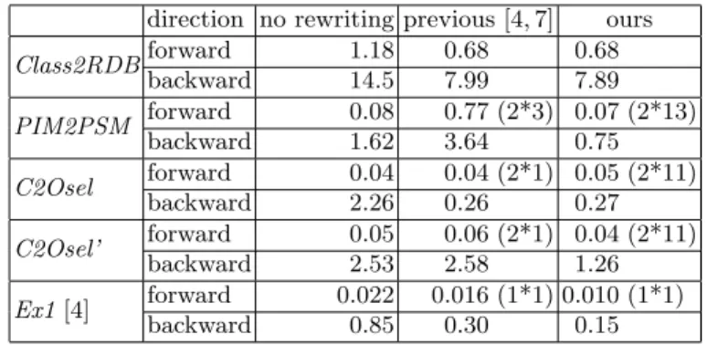
Table 1.Summary of Experiments (running time is in CPU seconds)
direction no rewriting previous [4, 7] ours
Class2RDBforward 1.18 0.68 0.68
backward 14.5 7.99 7.89
PIM2PSM forward 0.08 0.77 (2*3) 0.07 (2*13)
backward 1.62 3.64 0.75
C2Osel forward 0.04 0.04 (2*1) 0.05 (2*11)
backward 2.26 0.26 0.27
C2Osel’ forward 0.05 0.06 (2*1) 0.04 (2*11)
backward 2.53 2.58 1.26
Ex1[4] forward 0.022 0.016 (1*1) 0.010 (1*1)
backward 0.85 0.30 0.15
actually given. However, we suppose presence of modification would not make much difference in the running time. Running time of forward transformation in which rewriting is applied (last two columns) includes time for rewriting. Rewrit-ing took 0.006 CPU seconds at the worst case (PIM2PSM, ours). Class2RDB
stands for class diagram to table diagram transformation, PIM2PSMfor plat-form independent model to platplat-form specific model transplat-formation, C2Osel is for transformation of customer oriented database into order oriented database, followed by a simple selection, andEx1is the example that is extracted from our previous paper [7], which was borrowed from [4]. It is a composition of tworecs. Concrete plugging optimizations in this example can be traced in Sect. A.4 in the appendix.
The numbers in parentheses show how often the fusion transformation hap-pened. For example,PIM2PSM led to 3 fusions based on the second rule, and further enhanced rewriting led to 10 more fusion rule applications, all of which promoted to the first rule via proposed rewriting rule (2). Same promotions happened toC2Osel. Except forC2Osel’, a rtime optimization in which un-reachable parts are removed after every application ofrecis applied. Enhanced rewriting led to performance improvements in both forward and backward eval-uations, exceptC2Osel. Comparing “previous” with “no rewriting”, PIM2PSM
6
Related Work
Although some of our optimization rules were mentioned in [7], the relationship with static marker analysis was not covered in depth. Our optimization, based on the enhanced marker analysis in Sect. 3 , generalizes all the rules in [7] uniformly. In our previous paper [6], an implementation of rewriting optimizations was reported, but concrete strategies were not included in the paper.
Plugging constructor-only expressions into output marker expressions was discussed in the full (technical report) version of [3]. Their motivation was to express semantics of @at the constructor expression level and not graph data level as in [4]. It also mentioned renaming of markers to avoid capture of the output markers in cycle expressions7. We do attempt the same thing at the expression level but we argue here more formally.
Our rewriting rules are inspired by the technical report but the idea there is not yet exploited fully. They discussed the semantics of rec on the cycle
expressions, even when the body refered to graph variables, although marker environment that maps markers to connected subgraphs introduced there makes the semantics complex. But we could use the semantics to enhance rewriting rules forrecwithcyclearguments.
The journal version [4] mentioned run-time optimization in which, assuming top-down evaluation, only necessary components of structural recursion are ex-ecuted. For example, only&z1 component ofrecin&z1@rec( )( ) is evaluated. It is not applicable to our bidirectional settings which rely on bulk semantics [6]. A static analysis of UnCAL was described in [1], but the main motivation was to analyze the structure of graphs using graph schema, whereas our analysis focus on the connectivity of graphs.
7
Conclusion
In this paper, under the context of graph transformation using UnCAL graph algebra, enhanced static marker inference is first formalized. Fusion rule becomes more powerful thanks to the static marker analysis. Further rewriting rules based on this inference are also explored. Marker renaming for capture avoidance is formalized to support the rewriting rules. Under the context of bidirectional graph transformations [6], one of the advantage of static analysis is that we can keep implementation of bidirectional interpreter intact. The marker analysis and rewriting proposed can be considered as dead-code detection and elimination. We believe this technique can be used for other graph languages that based on graph model that have named connecting points like input/output nodes. Preliminary performance evaluation shows the usefulness of the optimization for various non-trivial transformations in the field of software engineering research. Future work under this context includes reasoning about effects on the back-ward updatability. Although rewriting is sound with respect to well-behavedness
7
In the technical report, cycle was represented by parallel equations, without cycle
of bidirectional transformations, backward transformation before and after rewriting may accept different update operations. Our conjecture is that sim-plified transformation accepts more updates, but this argument requires further discussions.
Acknowledgments We thank reviewers and Kazuyuki Asada for their thor-ough comments on the earlier versions of the paper. The research was supported in part by the Grand-Challenging Project on “Linguistic Foundation for Bidi-rectional Model Transformation” from the National Institute of Informatics, En-couragement of Young Scientists (B) of the Grant-in-Aid for Scientific Research No. 20700035 and Grant-in-Aid for Research Activity Start-up No. 22800003.
References
1. A. A. Bencz´ur and B. K´osa. Static analysis of structural recursion in semistructured databases and its consequences. InADBIS, pages 189–203, 2004.
2. P. Buneman, S. Davidson, M. Fernandez, and D. Suciu. Adding structure to un-structured data. InICDT, volume 1186 ofLNCS, pages 336–350, 1997.
3. P. Buneman, S. Davidson, G. Hillebrand, and D. Suciu. A query language and optimization techniques for unstructured data. InSIGMOD, pages 505–516, 1996. long version appears as U.Penn TR MS-CIS-96-09.
4. P. Buneman, M. F. Fernandez, and D. Suciu. UnQL: a query language and algebra for semistructured data based on structural recursion.VLDB J., 9(1):76–110, 2000. 5. K. Ehrig, E. Guerra, J. de Lara, L. Lengyel, T. Levendovszky, U. Prange, G. Taentzer, D. Varr´o, and S. Varr´o-Gyapay. Model transformation by graph transformation: A comparative study. Presented at MTiP 2005. http://www.inf.mit.bme.hu/FTSRG/Publications/varro/2005/mtip05.pdf, 2005. 6. S. Hidaka, Z. Hu, K. Inaba, H. Kato, K. Matsuda, and K. Nakano.
Bidirection-alizing graph transformations. In ACM SIGPLAN International Conference on Functional Programming, pages 205–216. ACM, 2010.
7. S. Hidaka, Z. Hu, H. Kato, and K. Nakano. Towards a compositional approach to model transformation for software development. InSAC 2009, pages 468–475, 2009.
8. G. Rozenberg, editor. Handbook of Graph Grammars and Computing by Graph Transformations, Volume 1: Foundations. World Scientific, 1997.
9. I. Sasano, Z. Hu, S. Hidaka, K. Inaba, H. Kato, and K. Nakano. Toward bidirec-tionalization of ATL with GRoundTram. InICMT, pages 138–151, June 2011. 10. P. Stevens. Bidirectional model transformations in QVT: Semantic issues and open
questions. InMoDELS 2007, pages 1–15, 2007.
A
Appendix
A.1 UnCAL Original Static Typing Rules
a∈ U
a:Label
ya label variable
y:Label
ta tree variable of typeTreeX
t:TreeX
{}:TreeX
X∈ X
X:TreeX
l:Label Q:TreeX
{l⇒Q}:TreeX
l1:Label l2:Label
l1=l2:Bool
l1:Label . . . ln:Label pa variable
p(l1, . . . , ln) :Bool
b:Bool Q1:TreeX Q2:TreeX
ifbthenQ1elseQ2:TreeX
Q1 :TreeY . . . Qm:TreeY (X1:=Q1, . . . , Xm:=Qm) :Tree{
X1,...,Xm}
Y
Q1:TreeX Q2 :TreeX
Q1∪Q2:TreeX
Q1:TreeX Q2:TreeXY
Q1@XQ2:TreeY
ylabel variable ttree variable of typeTreeY Q1:TreeXX Q2:TreeY
gextX(λ(y, t).Q1)(Q2) :TreeXX ·Y
Fig. 6.UnCAL Original Static Typing Rules (TR ver. of [2])
Note thatgextis an old notation of structural recursionrec.
A.2 Proof of Lemma 1 (Refined Type Safety)
The proof of Lemma 1 is based on induction on the structure of UnCAL expres-sion.
Proof. Base case:
Free variables: We assume that the type of free variables such as $db (input of the entire transformation) is available.
{}: By the definition of F[[{}]], outMarker(g) = ∅. By the type inference rule,
{}::DB∅. Therefore,∅=outMarker(g)⊆ Y=∅.
&y : outMarker(F[[&y]]) = {&y} and &y :: DB{{&y}. &y :: DB{&y}. Therefore,
{&y} =outMarker(g)⊆ Y ={&y}. Another nullrary constructor(): is treated similarly.
Inductive case:
{l:e}: Supposee::DBY,F[[e]] =g, andF[[{l:e}]] =g!. ThenoutMarker(g!) =
outMarker(g) by the definition ofF[[]] and {l:e}:: DBY by the type inference rule. Now suppose outMarker(g)⊆ Y as an induction hypothesis. Then we have outMarker(g) =outMarker(g!)⊆ Y.&m :=eis treated similarly.
F[[e1 ∪e2]] = g!. Then outMarker(g!) = outMarker(g1) ∪ outMarker(g2) by the definition of F[[]] and e1∪e2 :: DBY1∪Y2 by the type inference rule.
Now suppose outMarker(g1) ⊆ Y1 and outMarker(g2) ⊆ Y2 as induction hy-potheses. Then, by the property of the set union, we have outMarker(g!) =
outMarker(g1)∪outMarker(g2) ⊆ Y1∪ Y2. ⊕ is treated similarly because type inference and evaluation rules for the output markers are identical to those of
∪.
e1@e2: Suppose e1 :: DBXY1, e2 :: DBYZ2, F[[e1]] = g1, F[[e2]] = g2, and F[[e1@e2]] = g!. Then outMarker(g!) = outMarker(g2) by the definition of F[[]] and e1@e2 :: DBXY2 by the type inference rule. Observe that (after
connect-ing with matchconnect-ing input markers in g2) the output markers in g1 are ignored. Now suppose outMarker(g2) ⊆ Y2 as an induction hypothesis. Then we have outMarker(g!) =outMarker(g2)⊆ Y2.
cycle(e): Suppose e :: DBXY, F[[e]] = g, and F[[cycle(e)]] = g!. Then
outMarker(g!) = outMarker(g) \ inMarker(g) by the definition of F[[]] and
cycle(e) ::DBY\X by the type inference rule. Now supposeoutMarker(g)⊆ Y as an induction hypothesis. Then, sinceX =inMarker(g) by the exactness of input marker inference, we haveoutMarker(g!) =outMarker(g)\inMarker(g)⊆ Y \ X.
ifbthene1elsee2: Suppose e1::DBXY1,e2 ::DB
X
Y2,F[[e1]] =g1,F[[e2]] =g2,
and F[[ifb then e1 else e2]] = g!. Then, depending on the value of b, outMarker(g!) = outMarker(g
1) or outMarker(g!) = outMarker(g2) by the def-inition of F[[]] and ifbthene1elsee2 :: DBXY1∪Y2 by the type inference rule.
Now supposeoutMarker(g1)⊆ Y1andoutMarker(g2)⊆ Y2as induction hypothe-ses and do case analysis for b. Ifb =true, thenoutMarker(g!) =outMarker(g
1), so outMarker(g!) = outMarker(g
1) ⊆ Y1. For the other case, outMarker(g!) = outMarker(g2)⊆ Y2. For either case, by the property of the set union, we have outMarker(g!)⊆ Y1∪ Y2.
rec(λ($l,$t).eb)(ea) : Suppose ea :: DBXY, F[[ea]] = g, eb :: DBZZio, and
F[[rec(λ($l,$t).eb)(ea)]] =g!. Then,outMarker(g!) ={&y.&z |&y ∈outMarker(g), &z ∈ Z}by the definition ofF[[]] whereZ=Zi∪ Zo, andrec(λ($l,$t).eb)(ea) ::
DBX ·ZY·Z by the type inference rule. Now supposeoutMarker(g)⊆ Y as induction hypotheses. Then we have outMarker(g!) = {&y.&z | &y ∈ outMarker(g),&z ∈
Z} ⊆ {&y.&z |&y ∈ Y,&z ∈ Z}. Observe that F[[]] does not use set of markers produced by eb at run-time. Readers may wonder how the output markers are accessed via graph variable t, i.e., Y bound by rec affect the final result. Buneman et al. [4] does not explicitly mention, but it is natural to interpret as follows: UsuallyY is disjoint fromZiand therefore the output nodes marked by
Y are not connected to S1 node8. Therefore we can safely ignore suchY ine b.
Bound Variables: Variable $t is introduced byrec(λ($l,$t).eb)(ea) and $t is bound to each of the subgraphs reachable from each edge. Similarly to [4], the type inference rule estimates the output markers as identical to that for ea. So assuming type safety forea, type safety for $t immediately follows.
The above analysis covers all the expressions and thus conclude the proof. &'
8
A.3 Proof of Refinement of Marker Analysis
This section gives a proof of the property:
∀X∀Y,∃Y!⊇ Y(e::DBX
Y ⇔e:DBXY!)
that appeared in Sect. 3. Note that we writee:DBXY to denoteehas a typeDBXY
in the original type system.
(⇒)
Base case:
{}: According to the typing rules,{}::DB∅and{}:DBY. Since∅ ⊆ Y for any
Y, the property holds.
(): Treated similarly to{}.
&y :According to the typing rules,&y ::DB{&y} and&y :DBY for any Y 4&y. Since{&y} ⊆ Y, the property holds.
Inductive case:
{l:e}: Suppose e::DBY, e:DBY!, and {&y} ⊆ Y as the induction hypothesis. Then, according to the typing rule, {l:e}::DBY, and{l:e}:DBY!. So, the prop-erty holds.
&m :=eis treated similarly.
cycle(e): Suppose e::DBXX ∪Y, e:DBXX ∪Y!, and {&y} ⊆ Y as the induction hy-pothesis. We also assume X to be disjoint withY and Y!. Then, according to the typing rule,cycle(e)::DBXY and cycle(e):DBXY!. So, the property holds. e1∪e2: Suppose e1 :: DBXY1 and e2 :: DB
X
Y2, and suppose e1 : DB
X Y!
1 and e2:DBXY!
2 where Y1⊆ Y
!
1 and Y2⊆ Y2! as induction hypotheses. Then, accord-ing to the typaccord-ing rule, (e1∪e2) ::DBXY1∪Y2 and (e1∪e2) :DB
X
Y! whereY1! ⊆ Y! andY!
2⊆ Y!. SoY1∪ Y2⊆ Y!. Therefore, the property holds. e1⊕e2 andifbthene1elsee2 are treated similarly.
e1@e2: Fore1::DBXY ande2::DBY !
Z, supposee1:DBXY2 ande2:DB
Y!
Z! s.t.Y ⊆ Y2
andZ ⊆ Z! as induction hypotheses. Note that we assumeY ⊆ Y! for
compati-bility with the original type system, which require set of output markers of first operand and the input markers of the second operand to coincide, which means the former should be a subset of the latter,9i.e.,Y
2⊆ Y!. This means we cannot assumeY2to be arbitrary larger thanY, but only a set that is smaller or equal toY!. Then, according to the typing rule,e
1@e2::DBXZ ande2@e2:DBXZ!. Since
Z ⊆ Z!, the property holds.
rec(λ($l,$t).eb)(ea): Assumeea::DBXY andea! :DBXY! where Y ⊆ Y!. Spe-cial care is needed for eb: There is no use to have an output marker that is not included in the set of input marker in eb, since such excess output node is not connected to any other node. It is best explained by the rule of rec:
rec(λ($l,$t).eb)({l : d}) = eb[l/$l][d/$t]@rec(λ($l,$t).eb)(d). The set of
cor-9
Suppose the set of markers common to the two positions (output of the first operand and input of the second operand) which the original type system assigns isY##. Then
responding input markers is the set of input markers of eb itself. So we as-sume equal set of input and output markers for eb thuseb :: DBZZ. Then, we have rec(λ($l,$g).eb)(ea) :: DBX ·ZY·Z and rec(λ($l,$g).eb)(ea!) : DBX ·ZY!·Z. Since
Y · Z ⊆ Y!· Z, the property holds.
The above case analysis covers all the cases by the induction and thus con-cludes the proof. The opposite direction (⇐) can be proved similarly. &'
A.4 Concrete Rewriting Examples
This section shows input and output of optimizations used inEx1transformation appeared in Sect. 5. For input transformation Q1, our system producesQ2by applying first fusion rule. Previously the translation from Q2to Q3 was not automatic, but algorithm in Sect. 4 enables derivingQ3automatically.
Q3can be obtained by the plugging based rewriting rules. For example,
(&z1 := (&z1 := {"name": &z2}, &z2 := {"name": &z2})) @ (&z2 := &z1&z2, &z1 := &z1&z1)
becomes
&z1 := (&z1 := {"name": &z1&z2}, &z2 := {"name": &z1&z2}).
This pattern frequently appears after rec fusion because recoften appears in the pattern &z @rec( )( ) because from the UnQL surface syntax, only one component of structural recursion is necessary and the idiom&z@ implements this projection.
Q 1.
&z1@rec(\ ($L,$T). if $L = "name"
then (&z1 := {"name": &z2}, &z2 := {"name": &z2})
else (&z1 := &z1, &z2 := {$L: &z2})) (&z1@rec(\ ($L,$T).
if $L = "name"
then (&z1 := {"name": &z1}, &z2 := {"typeName": &z2}) else if $L = "primitiveDataType"
then (&z1 := {"primitiveDataType": &z2}, &z2 := {"primitiveDataType": &z2}) else (&z1 := {$L: &z1}, &z2 := {$L: &z2})) ($db))
Q 2.
&z1@(&z2 := &z1&z2, &z1 := &z1&z1)@ rec(\ ($Sa1,$T).
then (&z1 := (&z1 := {"name": &z2}, &z2 := {"name": &z2}) @ (&z2 := &z1&z2, &z1 := &z1&z1),
&z2 := (&z1 := &z1,
&z2 := {"typeName": &z2}) @ (&z2 := &z2&z2, &z1 := &z2&z1)) else if $Sa1 = "primitiveDataType"
then (&z1 := (&z1 := &z1,
&z2 := {"primitiveDataType": &z2}) @ (&z2 := &z2&z2, &z1 := &z2&z1),
&z2 := (&z1 := &z1,
&z2 := {"primitiveDataType": &z2}) @ (&z2 := &z2&z2, &z1 := &z2&z1))
else (&z1 := if $Sa1 = "name" then (&z1 := {"name": &z2},
&z2 := {"name": &z2})
else (&z1 := &z1, &z2 := {$Sa1: &z2}) @ (&z2 := &z1&z2, &z1 := &z1&z1),
&z2 := if $Sa1 = "name" then (&z1 := {"name": &z2},
&z2 := {"name": &z2})
else (&z1 := &z1, &z2 := {$Sa1: &z2}) @ (&z2 := &z2&z2, &z1 := &z2&z1)))($db)
Q 3.
&z1@(&z2 := &z1&z2, &z1 := &z1&z1)@ rec(\ ($Sa1,$T).
if $Sa1="name"
then (&z1&z1 := {"name": &z1&z2}, &z1&z2 := {"name": &z1&z2}, &z2&z1 := &z2&z1,
&z2&z2 := {"typeName": &z2&z2}) else if $Sa1 = "primitiveDataType"
then (&z1&z1 := &z2&z1,
&z1&z2 := {"primitiveDataType": &z2&z2}, &z2&z1 := &z2&z1,
&z2&z2 := {"primitiveDataType": &z2&z2} else (&z1 := if $Sa1 = "name"
then (&z1 := {"name": &z1&z2}, &z2 := {"name": &z1&z2}) else (&z1 := &z1&z1,
&z2 := {$Sa1: &z1&z2}), &z2 := if $Sa1 = "name"
then (&z1 := {"name": &z2&z2}, &z2 := {"name": &z2&z2}) else (&z1 := &z2&z1,
A.5 Proof of Remark 1 (Removal of Intermediate Graph)
The remark gives necessary condition of the removal of intermediate graphs via fusion rule applications.
In the following, the contextC with a hole!can be defined as
C::=!| {a:C} |C∪e|e∪C|C⊕e|e⊕C|&x :=C | C@e|e@C|cycle(C)
where e denotes UnCAL expressions which consist only of constructors, and
C[e!] denotes an expression that is made by replacing the hole inC by UnCAL expressione!.
case (i):$t2 does not appear free ine2. The contextC[] in the expression
rec(λ($l2,$t2).e2)(C[rec(λ($l1,$t1).e1)(e0)])
can be removed by the prior auxiliary rewriting rules summarized in Section 2.7 to form the following direct composition.
rec(λ($l2,$t2).e2)(rec(λ($l1,$t1).e1)(e0))
The first fusion rule will turn it into
rec(λ($l1,$t1).rec(λ($l2,$t2).e2)(e1))(e0).
Ife1 contains anotherrec, i.e.,
rec(λ($l1,$t1).rec(λ($l2,$t2).e2)(C![rec(λ($l0,$t0).e!)(. . .)]))(e0),
then, because $t2 still does not appear free ine2, this composition will also be turned into nesting
rec(λ($l1,$t1).rec(λ($l0,$t0).rec(λ($l2,$t2).e2)(e!)(. . .)))(e0)
using the prior rewriting rule of rec (to remove the context C!) and the first fusion rule. In this way, the body of the downstreamrecof the composition newly introduced by the fusion comes from the downstreamrecbefore fusion. So the condition to apply the first fusion rule is maintained. These process of fusion are repeated until all the generated compositions become nested. Therefore, all the intermediate results (compositions) are removed.
case (ii):$t2appears free in e2.
Suppose the contextC[] inrec(λ($l2,$t2).e2)(C[rec(λ($l1,$t1).e1)(e0)]) does not contain @ or cycle. Then, auxiliary rules of rec can remove the context and turn the expression into direct composition. Suppose our proposed marker analysis detects thate1 does not produce output markers. Then, the first fusion rule becomes applicable. At this point, possible composition that emerge as a result of fusion will be similar to the prior case, thus
If we can further determine that e! does not produce output markers, then the first fusion rule will be applied again. Therefore, the composition of recwhose body of the upstream only contains nesting of rec via contexts that do not include@or cycle, can be completely removed. &'
Let us examine, within case (ii) the subcase wheree1has output markers. If
![Fig. 6. UnCAL Original Static Typing Rules (TR ver. of [2])](https://thumb-ap.123doks.com/thumbv2/123deta/8631305.449571/20.918.271.673.276.547/fig-uncal-original-static-typing-rules-tr-ver.webp)
